Sunday, March 30, 2014

Looking at Measles Data in Project Tycho

Project Tycho includes data from all weekly notifiable disease reports for the United States dating back to 1888. These data are freely available to anybody interested. I wanted to play around with the data a bit, so I registered.

Measles

Measles are in level 2 data. These are standardized data for immediate use and include a large number of diseases, locations, and years. These data are not complete because standardization is ongoing. The data are retrieved as measles cases and while I know I should convert to cases per 100 000, I have not done so here.
The data come in wide format, so the first step is conversion to long format. The Northern Mariana Islands variable was created as logical, so I removed it. In addition, data from before 1927 seemed very sparse, so those are removed too.
r1 <- read.csv('MEASLES_Cases_1909-1982_20140323140631.csv',
    na.strings='-',
    skip=2)
r1 <- subset(r1,,-NORTHERN.MARIANA.ISLANDS)
r2 <- reshape(r1,
    varying=names(r1)[-c(1,2)],
    v.names='Cases',
    idvar=c('YEAR' , 'WEEK'),
    times=names(r1)[-c(1,2)],
    timevar='State',
    direction='long')
r2$State=factor(r2$State)
r3 <- r2[r2$YEAR>1927,]

Plotting

The first plot is total cases by year. It shows the drop in cases from vaccine (Licensed vaccines to prevent the disease became available in 1963. An improved measles vaccine became available in 1968.)
qplot(x=Year,
        y=x,
        data=with(r3,aggregate(Cases,list(Year=YEAR),function(x) sum(x,na.rm=TRUE))),


        ylab='Sum registered Measles Cases')+
    theme(text=element_text(family='Arial'))


Occurrence within a year by week

Winter and spring seems to be the periods in which most cases occur. The curve seems quite smooth, with a few small fluctuations. The transfer between week 52 and week 1 is a bit steep, which may be because I removed week 53 (only present in part of the years).

qplot(x=Week,
        y=x,
        data=with(r3[r3$WEEK!=53 & r3$YEAR<1963,],
            aggregate(Cases,list(Week=WEEK),
                function(x) sum(x,na.rm=TRUE))),
        ylab='Sum Registered Measles Cases',
        main='Measles 1928-1962')+
    theme(text=element_text(family='Arial'))

A more detailed look

Trying to understand why the week plot was not smooth, I made that plot with year facets. This revealed an interesting number of zeros, which are an artefact of processing method (remember, sum(c(NA,NA),na.rm=TRUE)=0). I do not know if the data distinguishes between 0 and '-'. There are 872 occurrences of 0 which suggests 0 is used. On the other hand, week 6 and 9 in 1980 in Arkansas each have one case, the other weeks from 1 to 22 are '-', which suggests 0 is not used. My feeling for that time part is that registration became lax after measles was under control and getting reliable data from the underlying documentation is a laborious task. 

References


Willem G. van Panhuis, John Grefenstette, Su Yon Jung, Nian Shong Chok, Anne Cross, Heather Eng, Bruce Y Lee, Vladimir Zadorozhny, Shawn Brown, Derek Cummings, Donald S. Burke. Contagious Diseases in the United States from 1888 to the present. NEJM 2013; 369(22): 2152-2158.

Sunday, March 23, 2014

Distribution Kinetics in JAGS

Chapter 19 of Rowland and Tozer (Clinical pharmacokinetics and pharmacodynamics, 4th edition) has distribution kinetics. I am examining problem 3. It is fairly easy, especially since essentially all formulas are on the same page under 'key relationships'. The only difficulty is that the formulas are symmetrical in λ1, c1 and λ2, cand they are exchanged between chains. For this I forced λ12. In addition, I do not really believe concentrations in the 4000 range are as accurately measured as those in the 5 range (in the period 1/2 hour to 1 hour, the decrease is about 80 units per minute). The measurement error is now proportional to concentration.

Data and model

C19SP3 <- data.frame(
    time=c(0.5,1,1.5,2,3,4,5,8,12,16,24,36,48),
    conc=c(4211,1793,808,405,168,122,101,88,67,51,30,13,6))

library(R2jags)
datain <- list(
    time=C19SP3$time,
    lconc=log(C19SP3$conc),
    n=nrow(C19SP3),
    dose=30*1000)

model1 <- function() {
  tau <- 1/pow(sigma,2)
  sigma ~ dunif(0,100)
  llambda1 ~dlnorm(.4,.1)
  cc1 ~ dlnorm(1,.01)
  llambda2 ~dlnorm(.4,.1)
  cc2 ~ dlnorm(1,.01)
  choice <- llambda1>llambda2
  c1 <- choice*cc1+(1-choice)*cc2
  c2 <- choice*cc2+(1-choice)*cc1
  lambda1 <- choice*llambda1+(1-choice)*llambda2
  lambda2 <- choice*llambda2+(1-choice)*llambda1
  
  for (i in 1:n) {
    pred[i] <- log(c1*exp(-lambda1*time[i]) +c2*exp(-lambda2*time[i]))
    lconc[i] ~ dnorm(pred[i],tau)
  }
  V1 <- dose/(c1+c2)
  AUC <- c1/lambda1+c2/lambda2
  CL <- dose/AUC
  V <- CL/lambda2
  Vss <- dose*(c1/pow(lambda1,2)+c2/pow(lambda2,2))/pow(AUC,2)
  }

parameters <- c('c1','c2','lambda1','lambda2' ,
   'V1','CL','Vss','AUC','V')
inits <- function() 
  list(
      sigma=rnorm(1,1,.1),
      cc1=9000,
      cc2=150)

jagsfit <- jags(datain, model=model1, 
    inits=inits, 
    parameters=parameters,progress.bar="gui",
    n.chains=4,n.iter=14000,n.burnin=5000,n.thin=2)

Results

Results same as in the book:
Inference for Bugs model at "C:\...5a.txt", fit using jags,
 4 chains, each with 14000 iterations (first 5000 discarded), n.thin = 2
 n.sims = 18000 iterations saved
          mu.vect sd.vect     2.5%      25%      50%       75%     97.5%  Rhat n.eff
AUC      7752.778 130.145 7498.102 7670.443 7751.138  7831.068  8016.879 1.002  3000
CL          3.871   0.065    3.742    3.831    3.870     3.911     4.001 1.002  3000
V          57.971   1.210   55.650   57.215   57.956    58.708    60.401 1.002  4000
V1          2.980   0.104    2.776    2.915    2.978     3.044     3.192 1.002  2800
Vss        18.038   0.600   16.865   17.662   18.029    18.404    19.251 1.002  3900
c1       9933.578 352.138 9253.229 9709.652 9927.037 10145.611 10659.610 1.002  2800
c2        147.197   2.412  142.333  145.734  147.207   148.659   152.069 1.001  5000
lambda1     1.790   0.028    1.734    1.772    1.790     1.807     1.847 1.002  2800
lambda2     0.067   0.001    0.065    0.066    0.067     0.067     0.068 1.001 10000
deviance  -59.366   4.394  -65.150  -62.608  -60.275   -57.058   -48.524 1.001  4100

For each parameter, n.eff is a crude measure of effective sample size,
and Rhat is the potential scale reduction factor (at convergence, Rhat=1).

DIC info (using the rule, pD = var(deviance)/2)
pD = 9.6 and DIC = -49.7
DIC is an estimate of expected predictive error (lower deviance is better).

Plot

The plot has narrow intervals, which is a reflection of the small intervals in the parameters.

Previous posts in this series:

Simple Pharmacokinetics with Jags

Sunday, March 16, 2014

PK calculations for infusion at constant rate

In this third PK posting I move to chapter 10, study problem 4 of Rowland and Tozer (Clinical pharmacokinetics and pharmacodynamics, 4th edition). In this problem one subject gets a 24 hours continuous dose. In many respects the Jags calculation is not very different from before, but the relation between parameters in the model and PK parameters is a bit different.

Data

Data is from infusion at constant rate, (1.5 µm/hr, but the calculations come out on the expected values with 1.5 µg/hr, and no molecular weight is given in the question) for 24 hours. Drug concentration (µg/L) in plasma is measured for 28 hours.
ch10sp4 <- data.frame(
    time=c(0,1,2,4,6,7.5,10.5,14,18,24,25,26,27,28),
    conc=c(0,4.2,14.5,21,23,19.8,22,20,18,21,18,11.6,7.1,4.1))

Model

The model is straightforward, but does suffer a bit from sensitivity of init values. The construction (time<24 and time>=24 is just a quick way to ensure that the up and down doing parts of the model sit at the correct spots in time.
library(R2jags)
datain <- as.list(ch10sp4)
datain$n <- nrow(ch10sp4)
datain$Rinf <- 1.5*1000
model1 <- function() {
  for (i in 1:n) {
    pred[i] <- Css*((1-exp(-k*time[i]))*(time[i]<24)
                  +exp(-k*(time[i]-24))*(time[i]>=24))
    conc[i] ~ dnorm(pred[i],tau)
  }
  tau <- 1/pow(sigma,2)
  sigma ~ dunif(0,100)
  Css <- Rinf/CL
  k <- CL/V
  V ~ dlnorm(2,.01)
  CL ~ dlnorm(1,.01)
  t0_5 <- log(2)/k
  Cssalt <- 3000/CL
  h1 <- Cssalt*(1-exp(-k))
  h2 <- Cssalt*(1-exp(-2*k))
  CLpermin <- CL/60
}

parameters <- c('k','CL','V','t0_5','Cssalt','h1','h2','Css','CLpermin')
inits <- function() 
  list(V=rlnorm(1,log(100),.1),CL=rlnorm(1,log(70),.1),sigma=rlnorm(1,1,.1))
jagsfit <- jags(datain, model=model1, 
    inits=inits, 
    parameters=parameters,progress.bar="gui",
    n.chains=4,n.iter=14000,n.burnin=5000,n.thin=2)
jagsfit
Inference for Bugs model at "C:/Users/.../modelf7824253314.txt", fit using jags,
 4 chains, each with 14000 iterations (first 5000 discarded), n.thin = 2
 n.sims = 18000 iterations saved
         mu.vect sd.vect    2.5%     25%     50%     75%   97.5%  Rhat n.eff
CL        68.021   3.252  62.069  65.902  67.845  69.932  75.065 1.001  6600
CLpermin   1.134   0.054   1.034   1.098   1.131   1.166   1.251 1.001  6600
Css       22.102   1.046  19.983  21.449  22.109  22.761  24.167 1.001  6600
Cssalt    44.204   2.092  39.965  42.899  44.218  45.522  48.333 1.001  6600
V        170.798  23.922 127.164 155.118 169.417 184.662 222.523 1.001 18000
h1        14.679   1.698  11.572  13.575  14.586  15.685  18.367 1.001 18000
h2        24.419   2.307  20.014  22.913  24.360  25.849  29.249 1.001 18000
k          0.406   0.058   0.306   0.368   0.401   0.438   0.536 1.001 18000
t0_5       1.742   0.243   1.293   1.583   1.730   1.886   2.267 1.001 18000
deviance  66.267   3.024  62.809  64.041  65.477  67.692  74.131 1.002  2000

For each parameter, n.eff is a crude measure of effective sample size,
and Rhat is the potential scale reduction factor (at convergence, Rhat=1).

DIC info (using the rule, pD = var(deviance)/2)
pD = 4.6 and DIC = 70.8
DIC is an estimate of expected predictive error (lower deviance is better).
Expected values: CL=1.2 L/min, t1/2=1.6 hr, V=164 L. The values are a bit off, it was given in the text that Css is 21 mg/L while the model finds 22.
Three additional parameters; Cssalt, h1, h2 correspond to part (c) of the question; what concentrations if the dosage is doubled. Expected answers: Cssalt=42, h1=14.8, h2=24.

Plot of the model

Last week I made a similar plot in classical R graphics, so this week using ggplot2. What I personally notice from a modelling perspective is that the narrowness of the band near time=0 which misses the point at time 1 h. The whole pattern of points there almost suggests a small delay and steeper increase (lower t1/2) would make for a better fit. Interestingly, the same can be seen in the decreasing part of the curve. From a data perspective, the wide variability around the plateau concentration may be important. Perhaps that particular variation is the cause of the steepness which I mentioned before. 

part (b) Is the curve in the up and down going part equally steep?

This requires a different model, since right now by definition they are equally shaped. The parameter k12, difference between k1 and k2, is the parameter of interest.
datain2 <- as.list(ch10sp4)
datain2$n <- nrow(ch10sp4)
model2 <- function() {
  for (i in 1:n) {
    pred[i] <- Css*((1-exp(-k1*time[i]))*(time[i]<24)
          +exp(-k2*(time[i]-24))*(time[i]>=24))
    conc[i] ~ dnorm(pred[i],tau)
  }
  tau <- 1/pow(sigma,2)
  sigma ~ dunif(0,100)
  k1 ~ dlnorm(0,0.001)
  k2 ~ dlnorm(0,0.001)
  Css ~ dnorm(21,.01)
  k12 <- k1-k2
}

parameters2 <- c('k1','k2','k12','Css')
jagsfit2 <- jags(datain2, model=model2,  
    parameters=parameters2,progress.bar="gui",
    n.chains=4,n.iter=14000,n.burnin=5000,n.thin=2)
Inference for Bugs model at "C:/Users/...modelf783e02e64.txt", fit using jags,
 4 chains, each with 14000 iterations (first 5000 discarded), n.thin = 2
 n.sims = 18000 iterations saved
         mu.vect sd.vect   2.5%    25%    50%    75%  97.5%  Rhat n.eff
Css       21.275   1.131 19.089 20.559 21.258 21.982 23.578 1.001  6800
k1         0.529   0.138  0.333  0.446  0.512  0.588  0.814 1.002  8300
k12        0.194   0.163 -0.074  0.099  0.182  0.272  0.520 1.015  3800
k2         0.334   0.068  0.215  0.291  0.329  0.374  0.480 1.001  8600
deviance  64.761   3.663 60.215 62.073 63.929 66.528 73.979 1.002  3900

For each parameter, n.eff is a crude measure of effective sample size,
and Rhat is the potential scale reduction factor (at convergence, Rhat=1).

DIC info (using the rule, pD = var(deviance)/2)
pD = 6.7 and DIC = 71.5

DIC is an estimate of expected predictive error (lower deviance is better).
It seems the difference is is just not large enough to be convincing, which is what was supposed to be found. Css has now decreased compared to the first model, closer to the value which was given.

Previous posts in this series:

Simple Pharmacokinetics with Jags

Sunday, March 9, 2014

PK calculation of IV and oral dosing in JAGS

I am examining IV and oral dosing of problem of Chapter 6, Question 6 or Roland and Tozer Rowland and Tozer (Clinical pharmacokinetics and pharmacodynamics, 4th edition) with Jags. In this problem one subject gets an IV and an oral dose.

Data

The data looks a bit irregular in the beginning of the curves, but seems well behaving nonetheless.
IV <- data.frame(
    time=c(0.33,0.5,0.67,1.5,2,4,6,10,16,24,32,48),
    conc=c(14.7,12.6,11,9,8.2,7.9,6.6,6.2,4.6,3.2,2.3,1.2))
Oral <- data.frame(
    time=c(0.5,1,1.5,2,4,6,10,16,24,32,48),
    conc=c(2.4,3.8,4.2,4.6,8.1,5.8,5.1,4.1,3,2.3,1.3))

plot(conc~time,data=IV[1:12,],log='y',col='blue',type='l')
with(Oral,lines(y=conc,x=time,col='red'))

Jags model

A n umber of questions are asked. It is the intention the model gives posteriors for all. Priors are on clearance, volume and a few other variables. The increasing part of the oral curve is modeled with a second compartment. The same is true for the sharp decreasing part of the IV model. However, where the increasing part is integral part of the PK calculations, the decreasing part of IV is subsequently ignored. I have been thinking of removing these first points, but in the end rather than using personal judgement I just modeled them so I could ignore them afterwards.
library(R2jags)
datain <- list(
    timeIV=IV$time,
    concIV=IV$conc,
    nIV=nrow(IV),
    doseIV=500,
    timeO=Oral$time,
    concO=Oral$conc,
    nO=nrow(Oral),
    doseO=500)

model1 <- function() {
  tau <- 1/pow(sigma,2)
  sigma ~ dunif(0,100)
# IV part
  kIV ~dnorm(.4,1)
  cIV ~ dlnorm(1,.01)
  for (i in 1:nIV) {
    predIV[i] <- c0*exp(-k*timeIV[i]) +cIV*exp(-kIV*timeIV[i])
    concIV[i] ~ dnorm(predIV[i],tau)
  }
  c0 <- doseIV/V
  V ~ dlnorm(2,.01)
  k <- CL/V
  CL ~ dlnorm(1,.01)
  AUCIV <- doseIV/CL+cIV/kIV
# oral part
  for (i in 1:nO) {
    predO[i] <- c0star*(exp(-k*timeO[i])-exp(-ka*timeO[i]))
    concO[i] ~ dnorm(predO[i],tau)
  }
  c0star <- doseO*(ka/(ka-k))*F/V
  AUCO <- c0star/k
  F ~ dunif(0,1)
  ka ~dnorm(.4,1)
  ta0_5 <- log(2) /ka
  t0_5 <- log(2)/k
}

parameters <- c('k','AUCIV','CL','V','t0_5','c0',
    'AUCO','F','ta0_5','ka','c0star',
    'kIV','cIV','predIV','predO')
inits <- function() 
  list(
      sigma=rnorm(1,1,.1),
      V=rnorm(1,25,1),
      kIV=rnorm(1,1,.1),
      cIV = rnorm(1,10,1),
      CL = rnorm(1,5,.5),
      F = runif(1,0.8,1),
      ka = rnorm(1,1,.1)
      )
jagsfit <- jags(datain, model=model1, 
    inits=inits, parameters=parameters,progress.bar="gui",
    n.chains=4,n.iter=14000,n.burnin=5000,n.thin=2)

Quality of fit

A plot of the posterior fit against the original data. It would seem we have an outlier.  
cin <- c(IV$conc,Oral$conc)
mIV <- sapply(1:ncol(jagsfit$BUGSoutput$sims.list$predIV),
    function(x) {
      mean(jagsfit$BUGSoutput$sims.list$predIV[,x])
    }
)
mO  <- sapply(1:ncol(jagsfit$BUGSoutput$sims.list$predO),
    function(x) {
      mean(jagsfit$BUGSoutput$sims.list$predO[,x])
    }
)      
plot(x=c(IV$conc,Oral$conc),y=c(IV$conc,Oral$conc)-c(mIV,mO))

Answers to questions

We have the following posteriors:
Inference for Bugs model at "C:/...BEnL/model1b6027171a7a.txt", fit using jags,
 4 chains, each with 14000 iterations (first 5000 discarded), n.thin = 2
 n.sims = 18000 iterations saved
           mu.vect sd.vect    2.5%     25%     50%     75%   97.5%  Rhat n.eff
AUCIV      219.959  16.975 189.743 208.636 218.846 230.210 256.836 1.002  2800
AUCO       200.468  15.102 171.908 190.523 199.987 209.928 231.722 1.001  7500
CL           2.346   0.182   1.995   2.226   2.344   2.461   2.712 1.002  2900
F            0.876   0.052   0.773   0.841   0.876   0.911   0.976 1.002  3200
V           56.463   2.752  51.610  54.583  56.280  58.112  62.465 1.002  3100
c0           8.876   0.426   8.005   8.604   8.884   9.160   9.688 1.002  3100
c0star       8.314   0.615   7.119   7.911   8.304   8.704   9.574 1.002  2000
cIV         11.229   2.485   7.029   9.511  11.003  12.654  16.804 1.003  1100
k            0.042   0.004   0.034   0.039   0.042   0.044   0.050 1.002  2200
kIV          2.064   0.510   1.132   1.704   2.041   2.396   3.126 1.004   800
ka           0.659   0.105   0.489   0.589   0.646   0.715   0.903 1.002  3200
predIV[1]   14.343   0.532  13.240  14.009  14.355  14.690  15.378 1.002  2500
predIV[2]   12.637   0.331  11.990  12.422  12.632  12.851  13.298 1.001 12000
predIV[3]   11.435   0.357  10.755  11.196  11.427  11.667  12.147 1.002  1600
predIV[4]    8.923   0.326   8.333   8.709   8.902   9.116   9.638 1.002  2900
predIV[5]    8.410   0.298   7.845   8.213   8.401   8.594   9.021 1.001 14000
predIV[6]    7.522   0.286   6.943   7.340   7.525   7.713   8.064 1.001  5900
predIV[7]    6.910   0.255   6.385   6.749   6.915   7.077   7.399 1.001  6200
predIV[8]    5.848   0.222   5.406   5.704   5.849   5.993   6.285 1.001  7800
predIV[9]    4.557   0.231   4.098   4.409   4.555   4.707   5.012 1.001  4500
predIV[10]   3.270   0.252   2.781   3.107   3.267   3.433   3.773 1.002  3100
predIV[11]   2.349   0.251   1.867   2.183   2.343   2.509   2.865 1.002  2700
predIV[12]   1.217   0.207   0.839   1.076   1.204   1.343   1.662 1.002  2500
predO[1]     2.138   0.214   1.750   1.995   2.124   2.263   2.599 1.001  8700
predO[2]     3.626   0.293   3.070   3.432   3.616   3.807   4.234 1.001 12000
predO[3]     4.653   0.306   4.050   4.452   4.652   4.847   5.264 1.001 16000
predO[4]     5.351   0.294   4.754   5.161   5.354   5.541   5.930 1.001 15000
predO[5]     6.375   0.277   5.801   6.202   6.383   6.562   6.894 1.002  3200
predO[6]     6.274   0.308   5.629   6.079   6.286   6.485   6.842 1.002  2800
predO[7]     5.455   0.292   4.852   5.270   5.461   5.648   6.018 1.002  3900
predO[8]     4.262   0.245   3.764   4.106   4.265   4.423   4.736 1.001  8600
predO[9]     3.057   0.227   2.605   2.910   3.058   3.207   3.504 1.001  8200
predO[10]    2.195   0.218   1.773   2.050   2.192   2.335   2.638 1.001  5200
predO[11]    1.135   0.180   0.805   1.013   1.127   1.247   1.519 1.002  3500
t0_5        16.798   1.713  13.830  15.655  16.652  17.770  20.617 1.002  2200
ta0_5        1.077   0.164   0.768   0.969   1.072   1.177   1.419 1.002  3200
deviance    38.082   5.042  30.832  34.357  37.207  40.918  50.060 1.003  1200

For each parameter, n.eff is a crude measure of effective sample size,
and Rhat is the potential scale reduction factor (at convergence, Rhat=1).

DIC info (using the rule, pD = var(deviance)/2)
pD = 12.7 and DIC = 50.8
DIC is an estimate of expected predictive error (lower deviance is better).
Expected answers:
t1/2=16.7 hr, AUCiv=217 mg-hr/L, AUCoral=191 mg-hr/L, CL=2.3 L/hr, V=55L, F=0.88
While the point estimates are close, the s.d. seem quite large.

Plot of models

A plot of the predicted concentration time curves, with confidence intervals. The wider intervals at the low end of the concentrations are due to the logarithmic scale.
tpred <- 0:48
simO <- sapply(1:jagsfit$BUGSoutput$n.sims,function(x) {
      jagsfit$BUGSoutput$sims.list$c0star[x]*
          (exp(-jagsfit$BUGSoutput$sims.list$k[x]*tpred)
            -exp(-jagsfit$BUGSoutput$sims.list$ka[x]*tpred))
    })
predO <- data.frame(mean=rowMeans(simO),sd=apply(simO,1,sd))

simIV <- sapply(1:jagsfit$BUGSoutput$n.sims,function(x) {
      jagsfit$BUGSoutput$sims.list$c0[x]*
          (exp(-jagsfit$BUGSoutput$sims.list$k[x]*tpred)
            +exp(-jagsfit$BUGSoutput$sims.list$kIV[x]*tpred))
    })
predIV <- data.frame(mean=rowMeans(simIV),sd=apply(simIV,1,sd))

plot(conc~time,data=IV[1:12,],log='y',col='blue',type='p',ylab='Concentration')
with(Oral,points(y=conc,x=time,col='red'))
lines(y=predO$mean,x=tpred,col='red',lty=1)
lines(y=predO$mean+1.96*predO$sd,x=tpred,col='red',lty=2)
lines(y=predO$mean-1.96*predO$sd,x=tpred,col='red',lty=2)
lines(y=predIV$mean,x=tpred,col='blue',lty=1)
lines(y=predIV$mean+1.96*predIV$sd,x=tpred,col='blue',lty=2)
lines(y=predIV$mean-1.96*predIV$sd,x=tpred,col='blue',lty=2)

Sunday, March 2, 2014

Simple Pharmacokinetics with Jags

In this post I want to analyze a first order pharmocokinetcs problem: the data of study problem 9, chapter 3 of Rowland and Tozer (Clinical pharmacokinetics and pharmacodynamics, 4th edition) with Jags. It is a surprising simple set of data, but still there is enough to play around with.

Data, model and analysis

The data is simple enough. One subject's concentration of cocaine (μg/L) in plasma as function of time, after a starting dose of 33 mg cocaine hydrochlorine. The model is simple enough, C=C0*exp(-k*t). A number of additional parameters are to be calculated, half-live (t1/2), Clearance (CL) and distribution volume (V). Additional information needed; molecular weight of cocaine 303 g/mol, cocaine hydrochloride 330 g/mol.
ch3sp9 <- data.frame(
    time=c(0.16,0.5,1,1.5,2,2.5,3),
    conc=c(170,122,74,45,28,17,10))

Bayesian model

This model has as feature that the (non-informative) priors are directly on the parameters which are in PK analysis important; distribution volume and clearance.
library(R2jags)
datain <- as.list(ch3sp9)
datain$n <- nrow(ch3sp9)
datain$dose <- 33*1000*303/340 # in ug cocaine
model1 <- function() {
  for (i in 1:n) {
    pred[i] <- c0*(exp(-k*time[i]))
    conc[i] ~ dnorm(pred[i],tau)
  }
  tau <- 1/pow(sigma,2)
  sigma ~ dunif(0,100)
  c0 <- dose/V
  V ~ dlnorm(2,.01)
  k <- CL/V
  CL ~ dlnorm(1,.01)
  AUC <- dose/CL
  t0_5 <- log(2)/k
}

parameters <- c('k','AUC','CL','V','t0_5')
inits <- function() 
  list(V=rlnorm(1,1,.1),CL=rlnorm(1,1,.1),sigma=rlnorm(1,1,.1))
jagsfit <- jags(datain, model=model1, 
    inits=inits, parameters=parameters,progress.bar="gui",
    n.chains=4,n.iter=14000,n.burnin=5000,n.thin=2)
jagsfit
Inference for Bugs model at "...", fit using jags,
 4 chains, each with 14000 iterations (first 5000 discarded), n.thin = 2
 n.sims = 18000 iterations saved
         mu.vect sd.vect    2.5%     25%     50%     75%   97.5%  Rhat n.eff
AUC      201.756   0.766 200.258 201.369 201.749 202.143 203.233 1.001 10000
CL       145.767   0.553 144.705 145.485 145.769 146.045 146.855 1.001 10000
V        147.568   0.496 146.607 147.320 147.569 147.819 148.515 1.002 18000
k          0.988   0.005   0.978   0.985   0.988   0.991   0.998 1.001 13000
t0_5       0.702   0.004   0.694   0.700   0.702   0.704   0.709 1.001 13000
deviance   6.769   4.166   2.236   3.801   5.682   8.557  17.538 1.001  6300

For each parameter, n.eff is a crude measure of effective sample size,
and Rhat is the potential scale reduction factor (at convergence, Rhat=1).

DIC info (using the rule, pD = var(deviance)/2)
pD = 8.7 and DIC = 15.4

DIC is an estimate of expected predictive error (lower deviance is better).
The expected answers according to the book are:
AUC=0.200 mg-hr/L, CL 147 L/hr, V=147 L, t1/2=0.7 hr. The numbers are slightly off compared to the book, but the expectation is that students use graph paper and a ruler.

Alternative Baysian model

This is more or less the same model, however log(conc) rather than conc is modelled.
datain2 <- as.list(ch3sp9)
datain2$conc <- log(datain2$conc)
datain2$n <- nrow(ch3sp9)
datain2$dose <- 33*1000*303/340 # in ug cocaine
model2 <- function() {
  for (i in 1:n) {
    pred[i] <- c0-k*time[i]
    conc[i] ~ dnorm(pred[i],tau)
  }
  tau <- 1/pow(sigma,2)
  sigma ~ dunif(0,100)
  c0 <- log(dose/V)
  V ~ dlnorm(2,.01)
  k <- CL/V
  CL ~ dlnorm(1,.01)
  AUC <- dose/CL
  t0_5 <- log(2)/k
}

parameters <- c('k','AUC','CL','V','t0_5')
inits <- function() 
  list(V=rlnorm(1,1,.1),CL=rlnorm(1,1,.1),sigma=rlnorm(1,1,.1))
jagsfit2 <- jags(datain2, model=model2, 
    inits=inits, parameters=parameters,progress.bar="gui",
    n.chains=4,n.iter=14000,n.burnin=5000,n.thin=2)
jagsfit2
Inference for Bugs model at "...93c1bb35a79.txt", fit using jags,
 4 chains, each with 14000 iterations (first 5000 discarded), n.thin = 2
 n.sims = 18000 iterations saved
         mu.vect sd.vect    2.5%     25%     50%     75%   97.5%  Rhat n.eff
AUC      201.817   1.857 198.159 200.825 201.806 202.812 205.446 1.002  2700
CL       145.732   1.343 143.147 145.005 145.728 146.440 148.410 1.002  2700
V        146.904   2.248 142.588 145.702 146.882 148.049 151.428 1.002  2200
k          0.992   0.009   0.975   0.988   0.992   0.997   1.009 1.002  3200
t0_5       0.699   0.006   0.687   0.695   0.699   0.702   0.711 1.002  3200
deviance -37.541   3.922 -42.015 -40.424 -38.553 -35.772 -27.287 1.002  1900

For each parameter, n.eff is a crude measure of effective sample size,
and Rhat is the potential scale reduction factor (at convergence, Rhat=1).

DIC info (using the rule, pD = var(deviance)/2)
pD = 7.7 and DIC = -29.9
DIC is an estimate of expected predictive error (lower deviance is better).
The results are fairly close to the first calculation, although the standard deviations are a bit larger. The question which is the better obviously depends on the expectations or knowledge on measurement error.  The book states the data is adapted from a paper (Chow et al., 1985, link to pdf), but that did not help me for this question.

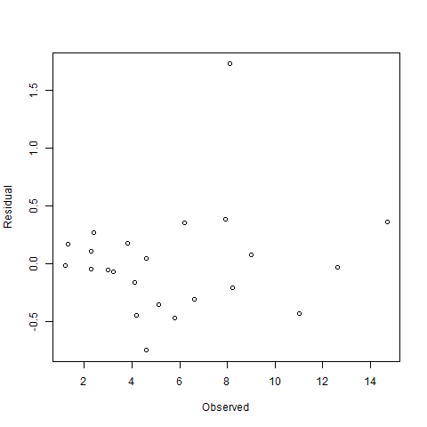
Looking at residuals

I find classic regression to be a bit more convenient to help me with the structure of the error.
l1 <- lm(log(conc) ~ time,data=ch3sp9)
l1
Call:
lm(formula = log(conc) ~ time, data = ch3sp9)

Coefficients:
(Intercept)         time  
     5.2994      -0.9922  
n1 <- nls(conc~c0*(exp(-k*time)),
    data=ch3sp9,
    start=c(k=0.1,c0=120))
n1

Nonlinear regression model
  model: conc ~ c0 * (exp(-k * time))
   data: ch3sp9
       k       c0 
  0.9878 199.2918 
 residual sum-of-squares: 0.5369

Number of iterations to convergence: 5 
Achieved convergence tolerance: 1.809e-07
par(mfrow=c(2,2))
plot(l1)

par(mfrow=c(1,1))
plot(x=predict(n1),y=resid(n1),main='nonlinear')
To me the non-linear model seems to have somewhat better behaving residuals.

Using a package

The package PKfit does offer these calculations. It is also completely menu operated, hence no code in this blog part. It does offer the possibility to specify error as shown here.
<< Weighting Schemes >> 
1: equal weight
2: 1/Cp
3: 1/Cp^2
The results are in line with before. 
               << Subject 1 >>


<< PK parameters obtained from Nelder-Mead Simplex algorithm >>

  Parameter       Value
1       kel   0.9883067
2        Vd 147.4714404

<< Residual sum-of-square (RSS) and final PK parameters with nls >>

  0:    0.31284706: 0.988307  147.471
  1:    0.31284252: 0.988292  147.474
  2:    0.31284252: 0.988292  147.474

<< Output >>

  Time Observed Calculated Wt. Residuals    AUC    AUMC
1 0.16      170  170.19433    -0.1943293     NA      NA
2 0.50      122  121.53930     0.4607031  49.64  14.994
3 1.00       74   74.24673    -0.2467286  98.64  48.744
4 1.50       45   45.29682    -0.2968236 128.39  84.119
5 2.00       28   27.64910     0.3508985 146.64 114.994
6 2.50       17   16.87096     0.1290408 157.89 139.619
7 3.00       10   10.29481    -0.2948107 164.64 157.744

<< AUC (0 to infinity) computed by trapezoidal rule >>

[1] 174.7585

<< AUMC (0 to infinity) computed by trapezoidal rule >>

[1] 198.3377


<< Akaike's Information Criterion (AIC) >>
[1] 8.961411

<< Log likelihood >>
'log Lik.' -1.480706 (df=3)

<< Schwarz's Bayesian Criterion (SBC/BIC) >>
[1] 8.799142


Formula: conc ~ modfun1(time, kel, Vd)

Parameters:
     Estimate Std. Error t value Pr(>|t|)    
kel 9.883e-01  3.518e-03   280.9 1.09e-11 ***
Vd  1.475e+02  3.231e-01   456.4 9.58e-13 ***
---
Signif. codes:  0 '***' 0.001 '**' 0.01 '*' 0.05 '.' 0.1 ' ' 1

Residual standard error: 0.3537 on 5 degrees of freedom

Algorithm "port", convergence message: both X-convergence and relative convergence (5)

Conclusion: distribution of parameters

In hindsight the first Bayesian model is the one I prefer. Since I wanted to have some idea about the distribution of the parameters I have added this plot.
par(mfrow=c(3,2))
lapply(1:length(jagsfit$BUGSoutput$sims.list),
    function(x) plot(density(jagsfit$BUGSoutput$sims.list[[x]]),
main=names(jagsfit$BUGSoutput$sims.list)[x]))