Sunday, December 28, 2014

A time series contest attempt

I saw the post a time series contest on Rob J Hyndman's blog. Since I am still wanting to play around with some bigger data sets, so I went to the source website https://drive.google.com/folderview?id=0BxmzB6Xm7Ga1MGxsdlMxbGllZnM&usp=sharing and got myself the data. One warning, if you are reading this to know how to get close to the winning result, you'd better stop now. I did not get even close.

Data

Data exists in two data sets, training and test. The data are time series, each of a 1000 time points and some summary statistics of these. The training set consists of 63530 samples, the test set an additional 77769. In practice this means 490 Mb and 600 Mb of memory. Not surprising, just prepping the data and dropping it in randomForest gives an out of memory error. The question then is how to preserve memory.
It seemed that my Windows 7 setup used more memory than my Suse 13.2 setup. The latter is quite fresh, while Win 7 has been used two years now, so there may be some useless crap which wants to be resident there. I did find that Chrome keeps part of itself resident, so switched that off (advanced setting). Other things which Win 7 has and Suse 13.2 misses are Google drive (it cannot be that hard to make it, but Google is dragging its heels) and a virus scanner, but there may be more.
This helped a bit, but this data gave me good reason to play a bit with dplyr's approach to store data in a database.
library(dplyr)
library(randomForest)
library(moments)

load('LATEST_0.2-TRAIN_SAMPLES-NEW_32_1000.saved')
my_db <- src_sqlite(path = tempfile(), create = TRUE)
#train_samples$class <- factor(train_samples$class)
train_samples$rowno <- 1:nrow(train_samples)
train <- copy_to(my_db,train_samples,indexes=list('rowno'))
rm(train_samples)

So, the code above reads the data and stores it in a SQLite database. At one point I made class a factor, but since SQLite does not have factors, this property is removed once the data is retrieved out of the database. I added a rowno variable. Some database engines have a function for row numbers, SQLite does not, and I need it to select records.
The key learning I got from this is related to the rowno variable. Once data is in the database, it just knows what is in the database and only understands its own flavour of SQL. Dplyr does a good job to make it as similar as possible to data.frames, but in the end one needs to have a basic understanding of SQL to get it to work.

Plot

The data has the property that part of it, the last n time points, are true samples. In this part the samples have an increase or decrease of 0.5%. The question is then what happens in the next part, further increase or decrease. The plot below shows the true samples of the first nine records. What is not obvious from the figure, is that the first two records have the same data, except for a different true part.  

First model

As a first step I tried a model with limited variables and only 10000 records. For this the x data has been compressed in two manners. From a time series perspective, where the ACF is used, and from trend perspective, where 10 points are used to capture general shape of the curves. The latter by using local regression (loess). Both these approaches are done on true data and all data. In addition, the summary variables provided in the data are used.
The result, an OOB error rate of 44%. Actually, this was a lucky run, I have had runs with error rates over 50%. I did not bother to check predictive capability.
mysel <- filter(train,rowno<10000) %>%
        select(.,-chart_length,-rowno) %>%
        collect()
yy <- factor(mysel$class)
vars <- as.matrix(select(mysel,var.1:var.1000))
leftp <- select(mysel,true_length:high_frq_true_samples)
rm(mysel)
myacf <- function(datain) {
    a1 <- acf(datain$y,plot=FALSE,lag.max=15)
    a1$acf[c(2,6,11,16),1,1]
}
myint <- function(datain) {
    ll <- loess(y ~x,data=datain)
    predict(ll,data.frame(x=seq(0,1,length.out=10)))
}

la <- lapply(1:nrow(vars),function(i) {
            allvar <- data.frame(x=seq(0,1,length.out=1000),y=vars[i,])
            usevar <- data.frame(x=seq(0,1,length.out=leftp$true_length[i]),
                    y=allvar$y[(1001-leftp$true_length[i]):1000])
            c(myacf(allvar),myacf(usevar),myint(allvar),myint(usevar))
        })
rm(vars)
rightp <- do.call(rbind,la)
colnames(rightp) <- c(
        paste('aacf',c(2,6,11,16),sep=''),
        paste('uacf',c(2,6,11,16),sep=''),
        paste('a',seq(1,10),sep=''),
        paste('u',seq(1,10),sep=''))

xblok <- as.matrix(cbind(leftp,rightp))
rf1 <-randomForest(
        x=xblok,
        y=yy,
        importance=TRUE)
rf1

Call:
 randomForest(x = xblok, y = yy, importance = TRUE)
               Type of random forest: classification
                     Number of trees: 500
No. of variables tried at each split: 6

        OOB estimate of  error rate: 44.21%
Confusion matrix:
     0    1 class.error
0 2291 2496   0.5214122
1 1925 3287   0.3693400

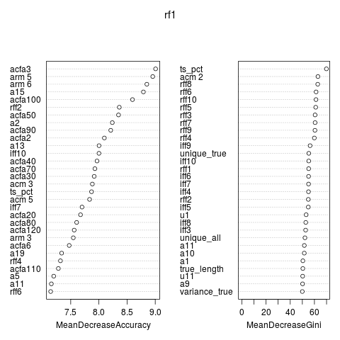
The plot shows the variable importance. Besides the variables provided the ACF seems important. Variables based on all time points seemed to work better than variables based on the true time series.

Second Model

In this model extra detail has been added to the all data variables. In addition extra momemnts of the data have been calculated. It did not help very much.
mysel <- filter(train,rowno<10000) %>%
        select(.,-chart_length,-rowno) %>%
        collect()
yy <- factor(mysel$class)
vars <- as.matrix(select(mysel,var.1:var.1000))
leftp <- select(mysel,true_length:high_frq_true_samples)
rm(mysel)
myacf <- function(datain,cc,lags) {
    a1 <- acf(datain$y,plot=FALSE,lag.max=max(lags)-1)
    a1 <- a1$acf[lags,1,1]
    names(a1) <- paste('acf',cc,lags,sep='')
    a1
}
myint <- function(datain,cc) {
    datain$y <- datain$y/mean(datain$y)
    ll <- loess(y ~x,data=datain)
    pp <- predict(ll,data.frame(x=seq(0,1,length.out=20)))
    names(pp) <- paste(cc,1:20,sep='')
    pp
}

la <- lapply(1:nrow(vars),function(i) {
            allvar <- data.frame(x=seq(0,1,length.out=1000),y=vars[i,])
            usevar <- data.frame(x=seq(0,1,length.out=leftp$true_length[i]),
                    y=allvar$y[(1001-leftp$true_length[i]):1000])
            acm <- all.moments(allvar$y,central=TRUE,order.max=5)[-1]
            names(acm) <- paste('acm',2:6)
            arm <- all.moments(allvar$y/mean(allvar$y),
                    central=FALSE,order.max=5)[-1]
            names(arm) <- paste('arm',2:6)
            ucm <- all.moments(usevar$y,central=TRUE,order.max=5)[-1]
            names(ucm) <- paste('ucm',2:6)
            urm <- all.moments(usevar$y/mean(usevar$y),
                    central=FALSE,order.max=5)[-1]
            names(urm) <- paste('urm',2:6)       
            ff <- fft(allvar$y[(1000-511):1000])[1:10]
            ff[is.na(ff)] <- 0
            rff <- Re(ff)
            iff <- Im(ff)
            names(rff) <- paste('rff',1:10,sep='')
            names(iff) <- paste('iff',1:10,sep='')
            c(myacf(allvar,'a',lags=c(2:10,seq(20,140,by=10))),
                    myint(allvar,'a'),
                    acm,
                    arm,
                    rff,
                    iff,
                    myacf(usevar,'u',seq(2,16,2)),
                    myint(usevar,'u')
            )
        })
#rm(vars)
rightp <- do.call(rbind,la)
xblok <- as.matrix(cbind(leftp,rightp))
rf1 <-randomForest(
        x=xblok,
        y=yy,
        importance=TRUE,
        nodesize=5)
rf1

Call:
 randomForest(x = xblok, y = yy, importance = TRUE)
               Type of random forest: classification
                     Number of trees: 500
No. of variables tried at each split: 10

        OOB estimate of  error rate: 42.76%
Confusion matrix:
     0    1 class.error
0 2245 2542   0.5310215
1 1734 3478   0.3326938


SVM

Just to try something else than a randomForest. But I notice some overfitting.
sv1 <- svm(x=xblok,
        y=yy
        )
sv1
Call:
svm.default(x = xblok, y = yy)

Parameters:
   SVM-Type:  C-classification
 SVM-Kernel:  radial
       cost:  1
      gamma:  0.009259259

Number of Support Vectors:  9998
table(predict(sv1),yy)

   yy
       0    1
  0 4776    2
  1   11 5210

A test set (rowno>50000 in the training table) did much worse
   ytest
       0    1
  0  547  580
  1 6254 6149

Sunday, December 21, 2014

Merry Christmas

Based on The DO loop, since I wanted a fractal Christmas tree and there is no point in inventing what has been made already. Besides, this is not the first time this year that I used R to do what has been done in SAS.

Code

# http://blogs.sas.com/content/iml/2012/12/14/a-fractal-christmas-tree/
# Each row is a 2x2 linear transformation 
# Christmas tree 
L <-  matrix(
    c(0.03,  0,     0  ,  0.1,
        0.85,  0.00,  0.00, 0.85,
        0.8,   0.00,  0.00, 0.8,
        0.2,  -0.08,  0.15, 0.22,
        -0.2,   0.08,  0.15, 0.22,
        0.25, -0.1,   0.12, 0.25,
        -0.2,   0.1,   0.12, 0.2),
    nrow=4)
# ... and each row is a translation vector
B <- matrix(
    c(0, 0,
        0, 1.5,
        0, 1.5,
        0, 0.85,
        0, 0.85,
        0, 0.3,
        0, 0.4),
    nrow=2)

prob = c(0.02, 0.6,.08, 0.07, 0.07, 0.07, 0.07)

# Iterate the discrete stochastic map 
N = 1e5 #5  #   number of iterations 
x = matrix(NA,nrow=2,ncol=N)
x[,1] = c(0,2)   # initial point
k <- sample(1:7,N,prob,replace=TRUE) # values 1-7 

for (i in 2:N) 
  x[,i] = crossprod(matrix(L[,k[i]],nrow=2),x[,i-1]) + B[,k[i]] # iterate 

# Plot the iteration history 
png('card.png')
par(bg='darkblue',mar=rep(0,4))    
plot(x=x[1,],y=x[2,],
    col=grep('green',colors(),value=TRUE),
    axes=FALSE,
    cex=.1,
    xlab='',
    ylab='' )#,pch='.')

bals <- sample(N,20)
points(x=x[1,bals],y=x[2,bals]-.1,
    col=c('red','blue','yellow','orange'),
    cex=2,
    pch=19
)
text(x=-.7,y=8,
    labels='Merry',
    adj=c(.5,.5),
    srt=45,
    vfont=c('script','plain'),
    cex=3,
    col='gold'
)
text(x=0.7,y=8,
    labels='Christmas',
    adj=c(.5,.5),
    srt=-45,
    vfont=c('script','plain'),
    cex=3,
    col='gold'
)

Sunday, December 14, 2014

Monthly Weather in Netherlands

When I downloaded the KNMI meteorological data, the intention was to do something which takes more than just the computers memory. While it is clearly not big data, at the very least 100 years of daily data is not small either. So I took along a load of extra variables to see what trouble I would run into. I did not run out of memory, but did make some figures.

Data

Data are acquired from KNMI. They have various sets of data, this page has a selection form which leads to the data used today. The data comes with a header explaining details, unfortunately in Dutch.

Plots

Just about everybody knows days are shorter in winter. What I never realized, even within that shorter day, we get less daylight. The short days are often so clouded, we don't get sun, meanwhile, in summer the sun does shine a bigger part of the daylight period.


In real hours sunshine this results in the following plot. December clearly has the darkest hours.
What we do get, not surprising since Dutch weather is fairly similar to English weather, is rain. Not continuous rain, most of the time it is dry, but still, autumn and winter do have days where it does not seem to stop. Autumn has the bad reputation for rain, but this plot makes winter look particular bad.
All this rain gives a load of humidity. This humidity in its turn, gives rise to a weather we name 'waterkoud'. It is above zero C but still quite cold outside. The humidity makes for air with a high heat capacity, hence one cools down quickly. Temperatures below zero can make for much nicer weather, but that can hamper traffic quite a lot. Most of the time it just doesn't freeze.
Code

library(plyr)
library(dplyr)
library(ggplot2)
r1 <- read.csv('KNMI_20141115.edited.txt')
Sys.setlocale(category = "LC_TIME", locale = "C")
r2 <- mutate(r1,
    date = as.Date(format(YYYYMMDD),'%Y%m%d'),
    month =factor(months(date,abbreviate=TRUE),
        levels=months(as.Date(
                paste('2014',
                    formatC(1:12,digits=2,width=2,flag='0'),
                    '01',sep='-')),
            abbreviate=TRUE)),
    yearf=factor(format(date,'%Y')),
    yearn=as.numeric(substr(YYYYMMDD,1,4)),
    day=format(date,'%e'))

g1 <- ggplot(r2,aes(x=month,y=SP))
g1 + geom_violin() +
        ylab('% of longest possible sunshine')

g1 <- ggplot(r2,aes(x=month,y=SQ/10))
g1 + geom_violin()  +
        ylab('Sunshine duration (h)')

g1 <- ggplot(r2,aes(x=month,y=DR/10))
g1 + geom_violin() +
        scale_y_continuous('Precipitation Duration (h)',
                breaks=c(0,6,12,18,24))

g1 <- ggplot(r2,aes(x=month,y=UG))
g1 + geom_violin() +
        ylab('Relative Humidity (%)')
 

g1 <- ggplot(r2,aes(x=month,y=TG/10))
g1 + geom_violin() +
        ylab('Temperature (C)')

Saturday, December 6, 2014

SAS PROC MCMC in R: Nonlinear Poisson Regression Models

In exercise 61.1 the problem is that the model has bad mixing. In the SAS manual the mixing is demonstrated after which a modified distribution is used to fix the model.
In this post the same problem is tackled in R; MCMCpack, RJags, RStan and LaplaceDemon. MCMCpack has quite some mixing problems, RStan seems to do best.

Data

To quote the SAS manual "This example shows how to analyze count data for calls to a technical support help line in the weeks immediately following a product release. (...) You can model the number of daily calls as a Poisson random variable, with the average number of calls modeled as a nonlinear function of the number of weeks that have elapsed since the product’s release. (...) During the first several weeks after a new product is released, the number of questions that technical support receives concerning the product increases in a sigmoidal fashion. The expression for the mean value in the classic Poisson regression involves the log link. There is some theoretical justification for this link, but with MCMC methodologies, you are not constrained to exploring only models that are computationally convenient. The number of calls to technical support tapers off after the initial release, so in this example you can use a logistic-type function to model the mean number of calls received weekly for the time period immediately following the initial release."
observed <- scan(text='
1 0 1 2 2 2 2 1 3 1 3 3
4 5 4 8 5 5 5 9 6 17 6 9
7 24 7 16 8 23 8 27',
    what=list(integer(),integer()),
    sep=' ',
)
names(observed) <- c('weeks','calls')
observed <- as.data.frame(observed)

Analysis

MCMCpack

The MCMCpack solution is derived from LaplacesDemon solution below. It is placed as first because it shows some of the problems with the mixing. As a change from LaplacesDemon, gamma could get negative, for which I made a -Inf likelihood.
library(MCMCpack)
MCMCfun <- function(parm) {
    names(parm) <- c('alpha','beta','gamma')
    if (parm['gamma']<0) return(-Inf)
    mu <-parm['gamma']*
        LaplacesDemon::invlogit(parm['alpha']+parm['beta']*observed$weeks)
    LL <- sum(dpois(observed$calls,mu,log=TRUE))
    LP <- LL+ dgamma(parm['gamma'],shape=3.4,scale=12,log=TRUE) +
        dnorm(parm['alpha'],-5,sd=.25,log=TRUE) +
        dnorm(parm['beta'],0.75,.5,log=TRUE)
    return(LP)
}
mcmcout <- MCMCmetrop1R(MCMCfun,
    c(alpha=-4,beta=1,gamma=2))

The figures show bad mixing. Parameters, especially Beta and Gamma, get stuck. There is quite some autocorrelation.
plot(mcmcout)
acf(mcmcout)
The cause is a nasty correlation between Beta and Gamma
pairs(as.data.frame(mcmcout))

LaplacesDemon

I chose an adaptive algorithm for LaplacesDemon. For the specs, the numbers are derived from the standard deviation of a previous run. Stepsize keeps reasonably constant through the latter part of run. The samples look much better than MCMCpack, although the mixing is not ideal either.
At a later stage I tried this same analysis with reflective Slice Sampler, however, that did was quite a bit more difficult and the end result was not better than this.
library('LaplacesDemon')
mon.names <- "LP"
parm.names <- c('alpha','beta','gamma')
PGF <- function(Data) c(rnorm(3,0,1))
N <-1
MyData <- list(mon.names=mon.names,
    parm.names=parm.names,
    PGF=PGF,
    calls=observed$calls,
    weeks=observed$weeks)
Model <- function(parm, Data)
{
    mu <-parm['gamma']*
        invlogit(parm['alpha']+parm['beta']*Data$weeks)
    LL <- sum(dpois(Data$calls,mu,log=TRUE))
    LP <- LL+ dgamma(parm['gamma'],shape=3.4,scale=12,log=TRUE) +
        dnorm(parm['alpha'],-5,sd=.25,log=TRUE) +
        dnorm(parm['beta'],0.75,.5,log=TRUE)
    Modelout <- list(LP=LP, Dev=-2*LL, Monitor=LP,
        yhat=mu,
        parm=parm)
    return(Modelout)
}

Initial.Values <- c(alpha=-4,beta=1,gamma=2) #GIV(Model, MyData, PGF=TRUE)
Fit1 <- LaplacesDemon(Model,
    Data=MyData,
    Initial.Values = Initial.Values,
    Algorithm = "AHMC",
    Specs = list(epsilon = c(.23,.2,13.5)/4,
        L = 2, Periodicity = 10),
    Iterations=40000,Status=2000   
)
BurnIn <- Fit1$Rec.BurnIn.Thinned
plot(Fit1, BurnIn, MyData, PDF=FALSE)

Jags

I do not think using one chain is advisable, especially since Jags makes more chains so easy. But in the spirit of this analysis I am using one. Coda plots are used since they are a bit more compact.
library(R2jags)
datain <- list(
    calls=observed$calls,
    weeks=observed$weeks,
    n=nrow(observed))
parameters <- c('alpha','beta','gamma')

jmodel <- function() {
    for (i in 1:n) {       
        mu[i] <- gamma*ilogit(alpha+beta*weeks[i])
        calls[i] ~ dpois(mu[i])
    }
    alpha ~ dnorm(-5,1/(.25*.25))
    gamma ~ dgamma(3.4,1/12)
    beta ~ dnorm(.75,1/(.5*.5))
}

jj <- jags(model.file=jmodel,
    data=datain,
    parameters=parameters,
    n.chains=1,
    inits=list(list(alpha=-4,beta=1,gamma=2))
    )

cc <- as.mcmc(jj$BUGSoutput$sims.array[,1,])

plot(cc)
acfplot(cc)

Stan

Stan probably does best handling this typical distribution. Again, one chain is only in the context of this posting.
library(rstan)
smodel <- '
    data {
    int <lower=1> n;
    int calls[n];
    real  weeks[n];
    }
    parameters {
    real Alpha;
    real Beta;
    real Gamma;
    }
    transformed parameters {
    vector[n] mu;
    for (i in 1:n) {
       mu[i] <- Gamma*inv_logit(Alpha+Beta*weeks[i]);
    }
    }
    model {
    calls ~ poisson(mu);
    Gamma ~ gamma(3.4,1./12.);
    Beta ~ normal(.75,.5);
    Alpha ~ normal(-5,.25);
    }
    '
fstan <- stan(model_code = smodel,
    data = datain,
    pars=c('Alpha','Beta','Gamma'),
    chains=1,
    init=list(list(Alpha=-4,Beta=1,Gamma=2)))

traceplot(fstan,inc_warmup=FALSE)

smc <- as.mcmc(as.matrix(fstan))
acfplot(smc)